Key Takeaways:

• What is PID Control: A PID controller (Proportional-Integral-Derivative) is a feedback control mechanism widely used in industry for its simplicity and robust performance. It continuously calculates an error value and adjusts process inputs to maintain the desired setpoint.

• P, I, D Components: The Proportional term reacts to current error, the Integral term accumulates past error, and the Derivative term predicts future error. Tuning these terms balances responsiveness, accuracy, and stability.

• Tuning Methods: Proper tuning is crucial. Common methods include manual trial-and-error and the Ziegler–Nichols tuning rules, which provide heuristic initial settings for the PID gains.

• Python Implementation: PID control can be implemented in code by iteratively calculating the P, I, and D contributions in each loop. We demonstrate a basic Python PID controller and simulate real-world examples (temperature, motor speed) with Matplotlib visualizations.

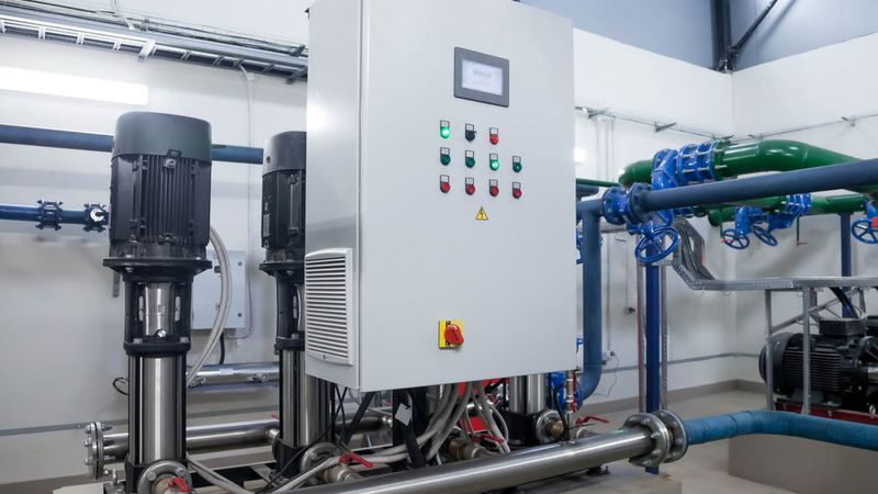
• Applications & Challenges: PID controllers are used in countless applications—from thermostats and automotive cruise control to robotics and industrial automation.

Introduction

Imagine a simple thermostat keeping your room at a steady temperature or a cruise control maintaining a car’s speed uphill and downhill. How do these systems automatically adjust to hit their target values? The answer lies in a fundamental feedback control strategy known as PID control. This article provides a comprehensive PID explained guide for engineers and students, demystifying how PID controllers work and how to apply them in practice. PID controllers are incredibly important in digital design, electronics, and industrial automation because they offer a reliable way to regulate processes with minimal error.

PID stands for Proportional-Integral-Derivative, referring to the three terms that make up the controller. It was first developed in the early 20th century and has since become the most common control algorithm in industrial applications. In essence, a PID controller continuously monitors a process variable (like temperature, speed, or pressure) and adjusts an input (such as heater power, motor voltage, valve position, etc.) to minimize the difference between the measured value and a desired setpoint. PID control operates as a closed-loop system, constantly correcting errors to maintain stability and accuracy.

What is PID Control?

PID control refers to a closed-loop feedback control system that uses a three-term controller to maintain a process variable at a desired setpoint. In a PID-controlled system, a sensor measures the current output (process variable), and the controller calculates the error as the difference between the setpoint and the measured value. 

The PID algorithm then computes a corrective control signal by combining three components: a proportional term (P), an integral term (I), and a derivative term (D). These terms adjust the output in proportion to the current error, accumulated past errors, and predicted future error trend, respectively. 

The control signal is applied to an actuator (such as a valve, heater, or motor) which influences the process, creating a feedback loop. By continuously updating the control input based on feedback, PID controllers can drive the system to the target setpoint and hold it steady despite disturbances.

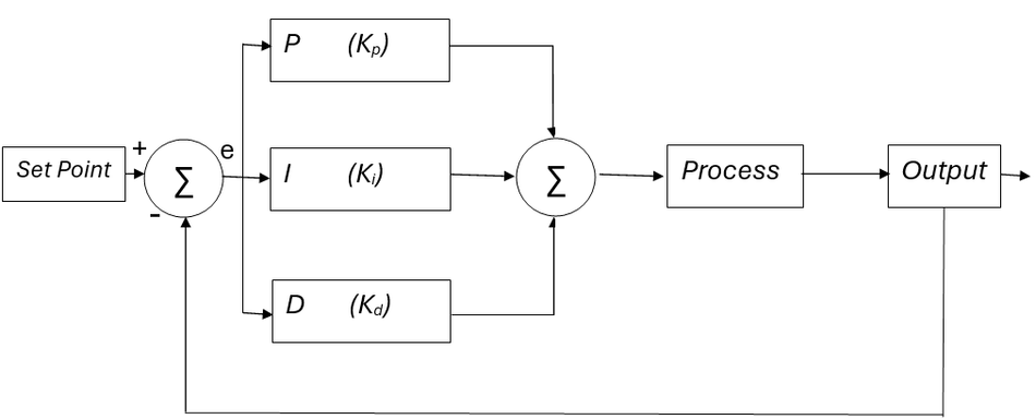
To put it simply, a PID controller “looks” at how far off the target we are right now (P), how long and how far we’ve been off in the past (I), and how fast the error is changing (D). By mathematically combining these three perspectives, the controller outputs a correction that pushes the process toward the setpoint stably and efficiently. This concept is illustrated in the standard PID control loop block diagram, where the error e(t) is fed into the P, I, and D blocks, and their outputs sum up to drive the process input.

Fig 1: A block diagram of a PID controller

PID controllers are so important because they offer a good balance of performance and simplicity for a wide range of control problems. They do not require an exact model of the system; instead, they rely on the feedback of the error itself. This makes PID broadly applicable – PID controllers are widely used in numerous applications requiring accurate, stable automatic control, such as temperature regulation, motor speed control, and industrial process management. 

They form the backbone of control loops in manufacturing, robotics, aerospace, electronics, and many other fields. Whenever you need to automatically maintain a parameter at some value (be it the temperature of a furnace, the speed of a conveyor, or the position of a servo motor), chances are a PID loop can do the job.

Suggested Reading: PID Controller & Loops: A Comprehensive Guide to Understanding and Implementation

Understanding Proportional, Integral, and Derivative Components

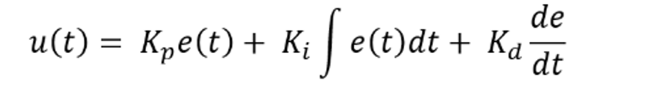
Now, let’s break down the three terms of PID control to understand their individual roles. The PID controller’s output at any given time t can be described by the formula:

Where:

u(t) = PID Control Value

 Kp = Proportional Gain

 e(t) = error value

 Ki = integral gain de= change in error

dt =change in time

Let’s examine each term:

• Proportional Term (P): This term produces an output that is proportional to the current error value. If the error is large, the proportional response is large; if the error is small, the response is small. The proportional gain Kpis a tuning parameter that scales this response. 

  • Effect: Proportional control drives the error toward zero by pushing back against the current error magnitude. However, using P alone typically leaves a steady-state error or offset. The process will stabilize when the proportional output balances the load, which often requires a non-zero error (for example, a simple proportional thermostat might stabilize a few degrees below the setpoint because some error is needed to drive the heater). Increasing Kp reduces this offset but too high a Kp can cause overshoot or oscillations.
    
    

• Integral Term (I): The integral term outputs an amount proportional to the accumulated error over time. It is computed as a running sum of past errors. The integral term grows whenever there is a persistent error, and it continues to increase until the error is eliminated. 

  • Effect: Integral control addresses the limitation of pure P control by driving the steady-state error to zero. It ensures that even a small residual error will accumulate and eventually be corrected by increasing the control output. However, the I term can introduce its own issues: it can make the system slower to respond (since it acts on accumulated error) and can cause overshoot if the integral builds up too much (more on integral windup in a later section). Tuning Ki sets how aggressively the controller tries to eliminate long-term error.
    
    

• Derivative Term (D): The derivative term produces an output proportional to the rate of change of the error.. It predicts where the error is heading by looking at how fast the error is increasing or decreasing. 

  • Effect: Derivative control provides a damping force – it counteracts rapid changes in the error, which helps reduce overshoot and oscillations. In other words, if the error is changing quickly, the D term adds a large correction in the opposite direction, anticipating future error. A well-tuned D term can improve the stability and settling time of the system. However, D control is very sensitive to noise in the feedback signal; even small measurement noise can have a large derivative, causing a noisy or jittery control output. For this reason, many practical PID controllers include a filter on the D term or implement what’s called “derivative on measurement” to mitigate noise amplification. Sometimes, the derivative gain Kd is set to 0 in systems that are very noisy or where derivative action is not beneficial, yielding a PI controller instead.
    
    

It’s the combination of P, I, and D actions that makes PID powerful. The P term gives an immediate push to reduce error, the I term slowly nudges the output to eliminate residual error, and the D term braces against sudden changes or overshooting. By tuning the gains Kp, Ki, and Kd, we can shape the controller’s behavior — from sluggish but stable (low gains) to fast but underdamped (high gains).

Tuning PID Controllers

Tuning a PID controller means finding the optimal values of Kp, KiKi, and Kd (or sometimes equivalent parameters like proportional band, integral time, derivative time) to achieve the desired system performance. Good tuning will result in a control loop that responds to setpoint changes or disturbances quickly and accurately, with minimal overshoot and steady-state error, and without oscillation. 

Several methods exist for PID tuning, ranging from theoretical calculations to empirical trial-and-error. Here are some common approaches:

• Manual Tuning (Trial and Error): Many engineers tune PID loops by hand, especially in the field. A typical process is to start with I and D terms at zero, increase Kp until the system responds adequately fast but without excessive overshoot, then introduce KiKi to eliminate steady-state error, and finally add a bit of Kd to reduce overshoot and oscillations. This approach requires iteration and experience, observing the system’s step response and adjusting gains to get a critically damped or slightly underdamped response as desired.

• Ziegler–Nichols Method: The Ziegler–Nichols tuning rules are a classic heuristic approach to find initial PID gains. There are two main Ziegler–Nichols methods: the oscillation (ultimate gain) method and the step response method. In the oscillation method, you first set Ki = 0 and Kd = 0, then gradually increase Kp until the system reaches the verge of instability and sustains consistent oscillations (this value of Kp is called the ultimate gain Ku, and the oscillation period is Tu). You then use formulas to set the gains based on Ku and Tu for a desired controller type (P, PI, or PID). The step response method (also by Ziegler and Nichols) involves analyzing the open-loop step response of the process (its delay and time constant) and using lookup formulas.

• Other Formal Methods: Over the years, many other tuning formulas and algorithms have been developed. The Cohen–Coon method is another classical approach for processes with dead time. More modern techniques involve software-based auto-tuning, where the control system itself applies a test signal and calculates appropriate PID settings. There are also optimization-based methods where you define a cost (like integrated error or settling time) and adjust gains to minimize it. For critical loops, engineers might linearize the system and design using frequency response methods (Bode plots) or pole placement to achieve certain stability margins and then translate those to PID gains.

• Tuning for Specific Behavior: Depending on the application, you might tune the PID for different objectives. For instance, in some systems, a little overshoot is acceptable if it means reaching the setpoint faster, whereas in others (say, controlling the temperature of a chemical reactor) overshoot must be minimized to avoid safety issues. You can deliberately tune the controller to be overdamped (no overshoot, slower response) or underdamped (some overshoot but faster settling). If the process dynamics change over time or with operating conditions, gain scheduling might be used – effectively using different PID gains in different regimes.

Suggested Reading: Mastering PID Tuning: The Comprehensive Guide

Practical Implementation in Python

To solidify understanding, let’s implement a simple PID controller in Python. This practical example will show how the PID algorithm works in code and how the controller affects a simulated process. We will create a basic PID loop and apply it to a hypothetical system (for example, controlling temperature or speed), then visualize the results.

Implementing a Basic PID Controller in Code

A PID controller can be implemented with just a few lines of code inside a loop. The controller’s job in each iteration is to read the current process variable (PV), compare it to the setpoint (SP), and output a control value. We maintain a state between iterations in the form of the integral of error (accumulated error) and the previous error (for the derivative calculation). Here’s a straightforward Python implementation:

def pid_controller(setpoint, pv, Kp, Ki, Kd, prev_error, integral, dt):
    error = setpoint - pv                      # current error
    integral += error * dt                     # accumulate error (for I term)
    derivative = (error - prev_error) / dt     # calculate error change rate (D term)
    output = Kp * error + Ki * integral + Kd * derivative  # PID formula
    return output, error, integral

This pid_controller function calculates the three-term contributions and returns the control output along with the updated error and integral for the next iteration. For a real system, you would apply output to your actuator (for example, setting a motor speed or heater power). The time step dt is the loop interval (in seconds). In practice, make sure to call the loop at a consistent interval or measure dt dynamically. Also note that the derivative term here is the finite difference of error; in a noisy system, you might want to low-pass filter this or limit it to avoid spikes.

Next, let’s simulate a simple system using this controller. We will consider a very basic process model: suppose our control output directly influences the rate of change of the process variable (this is like a first-order integrator process for simplicity, e.g., controlling velocity by adjusting acceleration). For example, if the output is a heating power, the temperature PV might increase proportionally to that power. We’ll simulate in discrete time: at each step, update the PV based on the output.

# Simulation parameters
setpoint = 100.0            # target value we want the PV to reach
pv = 0.0                    # initial process variable value
Kp, Ki, Kd = 1.0, 0.1, 0.05  # PID gains (example values)
prev_error = 0.0
integral = 0.0
dt = 0.1                    # time step (100 ms loop)


# Lists to store results for plotting
time_history = []
pv_history = []
sp_history = []
output_history = []


# Run the simulation for 100 time steps (10 seconds)
for i in range(100):
    control, error, integral = pid_controller(setpoint, pv, Kp, Ki, Kd, prev_error, integral, dt)
    # Apply control to the process (simple model: PV increases by control*dt)
    pv += control * dt  
    # Save data for analysis
    time_history.append(i * dt)
    pv_history.append(pv)
    sp_history.append(setpoint)
    output_history.append(control)
    # Update error for next loop
    prev_error = error

In this code, we initialize the PID gains and start with PV=0. The loop calls pid_controller each iteration to get the control output. We then update the pv by adding control * dt (this is a very simplified process model where the control acts like an acceleration or heating rate). We collect the PV, setpoint, and output values over time for later visualization.

After running this simulation, we can examine how the process variable responded over time:

import matplotlib.pyplot as plt
plt.figure()
plt.plot(time_history, pv_history, label="Process Variable (PV)")
plt.plot(time_history, sp_history, label="Setpoint (SP)", linestyle='--')
plt.xlabel("Time (seconds)")
plt.ylabel("Value")
plt.title("PID Control Simulation")
plt.legend()
plt.grid(True)
plt.show()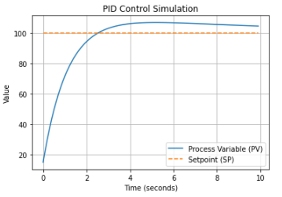

Fig 2: Response of a PID control system where a process variable traces a set point value

Running this would produce a plot of the PV moving towards the setpoint. With the example gains chosen above, the system will approach 100 and likely exhibit a slight overshoot before settling. The proportional term drives the initial rise, the integral term eliminates the final error, and the derivative term helps dampen the response.

In a real-world implementation, the process would be more complex than this simple integrator model – for instance, there might be inertia, lags, or higher-order dynamics. 

Real-World Example Use Cases

Let’s briefly consider a couple of real-world examples where we could apply PID control and how the Python implementation might look:

• Temperature Control (Thermostat/Oven): Suppose you have a heater, and you want to maintain an oven at 200°C. The process variable is the temperature a sensor measures, and the control output is the heater power (perhaps controlled via a PWM signal). A PID controller can adjust the heater output to minimize the difference between the current temperature and 200°C. The proportional term will heat stronger when the temperature is far from 200, the integral term will correct any steady error (e.g., if it’s consistently 5 degrees low, it will ramp up power over time), and the derivative term will reduce overshoot by cutting back heating as the temperature is rising quickly. In code, inside a loop, you’d do something like: 

output = pid_controller(200, current_temp, ...) 

and then use output to set the heater. You might also implement a safety cap on the output (0-100% power) and an anti-windup scheme for the integral if the heater saturates. Visualization of temperature vs time would show the temperature curve leveling off at 200 with minimal overshoot if tuned well.

• Motor Speed or Position Control: In robotics or automotive applications, PID is used to control motor speed or the position of a motor (for example, steering or a robotic arm joint). Here, the setpoint might be a desired RPM or angle, and the PV is measured via an encoder. The controller outputs a voltage or PWM duty cycle to the motor driver. For instance, cruise control in cars uses a PID loop: the setpoint is the desired speed, and the controller adjusts the throttle to minimize speed error. If the car goes uphill and slows down, the error increases, and PID adds throttle; if it goes downhill and speeds up, PID reduces throttle. In code, you would read the current speed, then 

output = pid_controller(target_speed, current_speed, Kp, Ki, Kd, ...) 

to compute a throttle adjustment. The derivative term helps prevent speed overshoot when cresting a hill, etc. Many robot balancing or trajectory-following problems also use PID loops on multiple motors.
Suggested Reading: Motion Control in Robotics: 4 Types of Motors for Industrial Robots

These examples show how versatile PID control is. Whether it’s temperature, speed, pressure, fluid flow, or any measurable quantity, if you can affect it with some input, a PID strategy can likely control it. Typical industrial processes like flow control valves, pressure regulators, and level controllers in tanks all use PID loops to maintain their set points. The same algorithm, with different tuning, works across many domains.

Common Challenges and Solutions

While PID controllers are conceptually simple, several practical challenges can arise when using them. Understanding these issues and knowing how to address them is key to successful PID tuning and implementation. Here are some common challenges and their solutions:

• Integrator Windup:

  • Problem: When the integral term accumulates a large error over time, it can lead to an overshoot and sluggish response. This often happens if the actuator saturates (hits a maximum or minimum limit) or after a large setpoint change. The integral keeps accumulating error even when the output can no longer increase, resulting in an “overwound” integral that must unwind later, causing the process variable to overshoot the target.

  • Solution: Techniques to prevent integral windup include integral clamping or reset windup prevention. For example, you can put limits on the integral term (not allowing it to grow beyond some bound). Another method is to disable or freeze the integral action when the error is very large or when the controller output is saturated. A more refined approach is back-calculation: adjusting the integral term based on the difference between the actual actuator output and the requested output to keep the integral in a realistic range. Most PID implementations in industrial controllers have an anti-windup mechanism for this reason. As a user, if you notice excessive overshoot after large setpoint steps, it’s a clue that integrator windup might be happening.

• Derivative Noise Sensitivity: 

  • Problem: The derivative term amplifies high-frequency noise in the error signal. If your sensor signal is noisy (which is common, e.g., with pressure sensors or accelerometers), the D term can fluctuate rapidly and make the control output jumpy. This noise can even destabilize an otherwise stable system.

  • Solution: A common practice is to filter the derivative term. Many PID controllers effectively implement a low-pass filter on the derivative calculation (for instance, using a moving average or a one-pole filter) to smooth out noise.

• Oscillation and Instability: 

  • Problem: If the PID gains are tuned improperly (for example, Kp too high, KiKi too high, or Kd too low to compensate), the control loop can become unstable and oscillate. You might see the process variable continually overshooting and undershooting the setpoint in a sustained way.

  • Solution: This typically means the loop needs to be tuned down. Reducing Kp or Ki will usually help stabilize an oscillatory system. Ensure that the derivative action Kd is sufficient to provide damping. Another cause for oscillation can be a significant time delay in the system (dead time) which makes PID control harder. In such cases, using a small derivative or a smith predictor (model-based approach) can help. The Ziegler–Nichols ultimate gain method leverages the onset of oscillation to tune; however, that initial oscillation should be avoided in normal operation. If a loop oscillates, retune by lowering gains or consider if the process has changed (e.g., different load conditions).

• Controller Saturation: 

  • Problem: The PID output may demand an action beyond the physical capabilities of the actuator (e.g., asking a heater for 120% power or a motor for more voltage than available). This saturates the output at its max/min. Saturation ties into integrator windup, as mentioned. It also effectively turns the control loop open (since further increases in error can’t increase output if it’s already maxed out).

  • Solution: Always limit the output to a  feasible range and incorporate that into your design. Use anti-windup, as discussed, to handle the integrator during saturation.

• Changing Dynamics: 

  • Problem: Sometimes, the process behavior changes under different conditions. For example, a vehicle handles differently uphill vs downhill, or a chemical process responds slower when nearing a threshold. A single set of PID gains might not work optimally for all scenarios. 

  • Solution: Techniques like gain scheduling can be used, where you change PID gains on the fly according to the operating region or known conditions. Adaptive PID controllers can also adjust their gains based on performance feedback. If dynamics vary widely, you might split the control into multiple PID controllers for different ranges or consider advanced adaptive control schemes.

Applications of PID in Industry

PID controllers are ubiquitous in engineering and industry. It’s not an exaggeration to say that a large majority of control loops in industrial processes use PID or a variant of it. Here are some notable application areas and examples:

• Manufacturing Process Control: In chemical plants and refineries, PID loops regulate temperature, pressure, flow, and level. For instance, controlling the pressure in a reactor or the flow rate of a fluid in a pipeline is typically done with a PID controller adjusting a control valve. The setpoint is the desired pressure or flow, and the PID manipulates the valve opening. The reason PID is so popular here is that it’s model-independent and can be tuned on-site for the specific process unit. Even with the rise of advanced control techniques, PID remains the most widely used technology for maintaining control over business-critical production processes. 

• Motion Control and Robotics: Almost every motion control system uses PID feedback loops. DC motor speed controllers, servo motor position controllers, and robot arm joint controllers often use PID algorithms. For example, a CNC machine uses PID loops to control the position of each axis precisely. In drones or aircraft autopilots, PID controllers help maintain attitude and altitude. Robotics often employs multiple PIDs – one for each motor – and sometimes nested PIDs (e.g., an outer loop for position and an inner loop for motor torque). The popularity of PID in robotics comes from its ease of implementation on microcontrollers and its ability to provide stable and smooth control with minimal computational resources.

Fig 3: Motion control applications such as robotic videography require high-precision motor control possible with PID controllers

• Automotive and Aerospace: Cruise control in cars, as mentioned, is a textbook example of PID control in action. Engine control systems also use PID loops (like in maintaining engine idle speed, where the controller adjusts throttle or fuel to keep the RPM at target). In aerospace, auto-throttle systems, autopilot altitude hold, and environmental control systems use PID regulators. For instance, an autopilot might use a PID to maintain a certain pitch angle by adjusting the elevator control surface.

• Power Systems: PID controllers are used in power electronics and power systems, such as regulating the output of power supplies (voltage regulation loops in a DC power supply or an inverter use PID to maintain constant output despite load changes). In larger power grid systems, PID controllers can help control generator output, frequency, and voltage regulators.

• Embedded Systems (Temperature, Lighting, etc.): On a smaller scale, even consumer devices use PID. Your oven or refrigerator likely has a PID temperature controller. PID algorithms are also found in 3D printers (to control nozzle temperature and motion axes), climate control systems (HVAC maintaining room temperature), and so on. For example, a simple homebrew PID might be used to control the temperature of a soldering iron or an incubator, where the heater is controlled via PWM.

Suggested Reading: Microcontroller Programming: Mastering the Foundation of Embedded Systems

Conclusion

This article provided a comprehensive explanation of PID controllers, starting with their fundamental principles and delving into the proportional, integral, and derivative components. We illustrated how these elements combine to correct process errors and achieve excellent control performance through proper tuning. A Python implementation demonstrated the PID loop's ability to drive a process variable to its setpoint, showcasing concepts like overshoot and damping.

The core strength of PID controllers lies in their power and relative simplicity, translating theoretical calculus into straightforward computations easily implemented in various platforms. While tuning presents a common challenge, established methods and systematic approaches enable the creation of well-behaved control loops. Furthermore, we addressed practical considerations like integrator windup and derivative noise sensitivity. The enduring relevance of PID control, evident in its widespread use across diverse applications, highlights its reliability and adaptability, even with the rise of advanced control techniques. Mastering PID control remains a valuable skill for engineers across disciplines, providing a foundational solution to numerous engineering challenges.

FAQ

1. What does PID stand for, and what is a PID controller?

PID stands for Proportional-Integral-Derivative. It refers to a three-term controller algorithm used in feedback control systems. A PID controller continuously calculates an error value as the difference between a desired setpoint and a measured process variable, then adjusts the control input (output) using the proportional, integral, and derivative terms to correct that error. In simple terms, a PID controller automatically tunes an input to drive a system’s output to the target value with minimal steady-state error and oscillation.

2. How does a PID controller work in practice?

A PID controller works by combining three actions: the Proportional action adjusts the output in proportion to the current error (if you’re far from the setpoint, it gives a strong push; if you’re close, a gentle push), the Integral action adjusts the output based on the accumulation of past errors (correcting any residual offset by adding up error over time), and the Derivative action adjusts the output based on the rate of change of the error (providing a braking force if the error is changing quickly, to avoid overshoot). These three contributions are summed to form the control signal. In practice, you measure the process variable (e.g., temperature, speed), compute the error, apply the PID formula to each loop iteration, and output the result to the actuator. Over time, this feedback loop drives the error toward zero and maintains the process at the setpoint.

3. How do I tune a PID controller?

Tuning a PID controller means selecting the gains Kp, Ki, and Kd so that the system responds well. There are a few approaches:

• Manual tuning: Increase Kp until you get a responsive (but not wildly oscillating) behavior. Then, introduce Ki to eliminate steady-state error (too much Ki can cause oscillation, so add it slowly). Finally, add Kd to reduce overshoot and settling time. Adjust each as needed while observing the response.

• Ziegler–Nichols method: Set KiKi and Kd to 0, raise Kp until the system just starts to oscillate (find Ku). Note the oscillation period Tu. Then, set Kp, Ki, and Kd according to the formula. 

• Software/auto-tuning: Some controllers can perform a tune themselves by injecting a test signal. Tools and software (like MATLAB’s PID tuner or microcontroller libraries) can auto-tune by measuring response. After an initial tuning, you usually fine-tune by trial and error. Good tuning achieves a balance: fast response, minimal overshoot, and no steady-state error.

4. What are common applications of PID controllers?

PID controllers are extremely common. Industrial process control (temperature, pressure, flow, level in chemical plants, manufacturing) heavily uses PIDs. Motor control is another area – for example, controlling the speed of a motor or the position of a servo (robots, CNC machines, hard drive head positioning, etc.). Automotive examples include cruise control (maintaining vehicle speed)  and engine idle speed control. Aerospace uses PIDs in autopilots for altitude, attitude, and throttle control. Even consumer devices like ovens, refrigerators, and air conditioners use PID loops for temperature control. Essentially, any system where you have a measurable output and an input you can adjust is a candidate for PID control if you need to maintain the output at some target.

5. What is the difference between P, PI, and PID control?

The difference lies in which of the three terms are used:

• P (Proportional) control: Uses only the proportional term. It reacts to current error. It’s simple but usually leaves a steady-state error (offset) because once at setpoint, the output would drop to zero and often, the process settles with some error.

• PI (Proportional-Integral) control: Uses P and I terms. The integral term accumulates error and drives the offset to zero, so PI controllers can eliminate steady-state error. Most slow processes (like temperature control) use PI if derivative action is not needed. The lack of D means it might be slower to settle and can overshoot more, but it’s simpler and less sensitive to noise.

• PID (Proportional-Integral-Derivative) control: Uses all three terms. The derivative term adds predictive damping, which can significantly reduce overshoot and improve settling time in fast or oscillatory systems. PID is generally used when you need quick response but also want to minimize overshoot or oscillation (for example, motion control systems). However, PID is also more sensitive to noise and more complex to tune than PI. There’s also PD control (P and D only, no I) which is sometimes used in motion control to get fast response without steady-state error elimination (or when steady-state error can be handled by another mechanism or is acceptable).

6. What is integral windup and how do I prevent it?

Integral windup is a situation where the integral term in a PID controller accumulates a large error during conditions when the controller can’t correct it (for instance, during a large setpoint change or when the actuator is saturated at a limit). When the error eventually reduces, the integral term may be so large that it causes the controller to overshoot the setpoint significantly since the integrator needs to “unwind.” In effect, the controller output remains too high (or too low) for a while because the integral has stored a big value. To prevent windup, you can:

• Temporarily disable or freeze the integral term if the control output is at an extreme limit or if the error is very large.

• Put limits on the integral term (e.g., don’t let it grow beyond some threshold).

• Use a technique called anti-windup or integrator clamping where you bleed off or adjust the integrator when the output saturates .
   Most PID controller libraries and hardware have anti-windup mechanisms you can enable. By preventing the integral from growing without bound, you ensure the controller can recover quickly after large disturbances or setpoint changes.

7. Why is PID still so widely used in control systems?

PID remains popular because of its simplicity, effectiveness, and versatility. It doesn’t require a detailed mathematical model of the system (unlike many advanced control techniques) and yet can be tuned to get very good performance for the majority of processes. Practically, PID controllers are easy to implement (just a few lines of code or simple analog circuits) and engineers are very familiar with them. Over decades, a lot of knowledge and best practices have been developed to make PID tuning easier and to handle its known issues. It’s also computationally light, which is great for embedded systems. While advanced methods (adaptive control, model predictive control, AI-based control) exist, they are often unnecessary for most tasks when a PID does the job well. As a result, PID is found everywhere in industry and will likely remain the cornerstone of control engineering for years to come 

References 

1. The PID Controller & Theory Explained - NI

2. PID Controller: Types, What It Is & How It Works | Omega

3. Proportional–integral–derivative controller - Wikipedia

4. Ziegler–Nichols method - Wikipedia

5. FEBRUARY 2011 – PID TUNING FOR ALLEN-BRADLEY PLCS - Control Station